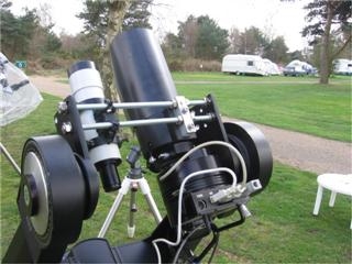
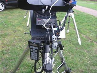
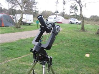
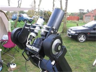
Time Delay Integration a.k.a Drift Scanning

[et_pb_section bb_built="1"][et_pb_row][et_pb_column type="4_4"][et_pb_text _builder_version="3.9"]

What is Drift Scanning?

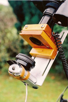
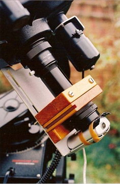
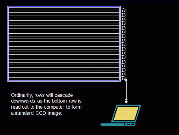
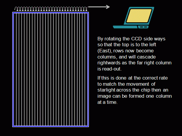
If you try to take an image on an un-driven mount the stars will trail as the Earth rotates. Now imagine a star on a CCD, it will move from pixel to pixel producing a line rather than a point source. Now if we could move the image on the CCD at the same rate as the star is moving across it, we would be able to keep the star as a point source on the image even though it is moving across the CCD. The total time of the exposure would be the time it takes for the star to cross the CCD.

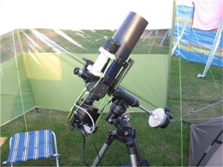
Drift scanning employs a special feature of some CCD cameras, such as the SBIG ST-7XME CCD camera. Data on these CCD’s can be read out one line at a time, and when this is done, the the whole image is shifted, so as the bottom line is read out to the computer, all the other lines move down. If the CCD is rotated correctly it can be read out in the same direction a star travels across it, and if it is read out at the same speed as a star travels across the chip from pixel to pixel we will have pin point stars.

[/et_pb_text][/et_pb_column][/et_pb_row][et_pb_row][et_pb_column type="1_2"][et_pb_text admin_label="image" _builder_version="3.9"]

Driftscan01

[/et_pb_text][/et_pb_column][et_pb_column type="1_2"][et_pb_text admin_label="image" _builder_version="3.9"]

Driftscan02

[/et_pb_text][/et_pb_column][/et_pb_row][et_pb_row][et_pb_column type="4_4"][et_pb_text _builder_version="3.9"]

Why Bother

This seems a lot of bother when you could simply drive your mount, so why do it? Well by employing this method it is possible to produce very long images like the one below.

[/et_pb_text][et_pb_code admin_label="Youtube video" _builder_version="3.9"]<div style="position:relative;height:0;padding-bottom:81%"><iframe src="https://www.youtube.com/embed/4CceDdn5pmo?ecver=2" style="position:absolute;width:100%;height:100%;left:0" width="444" height="360" frameborder="0" allow="autoplay; encrypted-media" allowfullscreen></iframe></div>[/et_pb_code][/et_pb_column][/et_pb_row][et_pb_row][et_pb_column type="1_2"][et_pb_text _builder_version="3.9"]

Software

Two pieces of software are available for drift scanning;
Maxim DL (commercial ~$199 to $665)
WinScan 2.33 (freeware) www.driftscan.com

Pros and Cons

The Pros
  • The set-up does not have to be driven
  • Is simple (?)(!)
  • Wide field shots can be taken
  • Polar alignment is not required
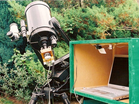
  • Little equipment is needed:CCD camera Telescope / Long Lens
  • Tripod
  • Laptop
The Cons:
  • Pointing, because the image will be a strip of the sky so when you start you won't be on your target(s)
  • Obtaining accurate parallel/perpendicular alignment
  • Focussing is a nightmare if not on a driven mount, but is achievable

Setting up the software

Only works with certain focal lengths
Differential trailing can be a problem
Viewing the images (they are large up to 32,000 pixels wide not many viewers will display them

[/et_pb_text][/et_pb_column][et_pb_column type="1_2"][et_pb_text admin_label="image" _builder_version="3.9"]

driftscan03

[/et_pb_text][/et_pb_column][/et_pb_row][/et_pb_section]

Crayford Eyepiece Mount (Crayford Focuser)

[et_pb_section bb_built="1"][et_pb_row][et_pb_column type="4_4"][et_pb_text _builder_version="3.9"]

Introduction

Designed and donated to the world by telescope maker and former member John Wall.

The design has two principle features:-

  • Restriction of movement of the eyepiece focusing tube to one degree of motion - which is linear - and a secondary motion of rotation.
  • The rapid interchange of eyepieces having different magnifications.

[/et_pb_text][/et_pb_column][/et_pb_row][et_pb_row][et_pb_column type="1_3"][et_pb_text _builder_version="3.9"]

CEMdrawing

[/et_pb_text][/et_pb_column][et_pb_column type="2_3"][et_pb_text _builder_version="3.9"]

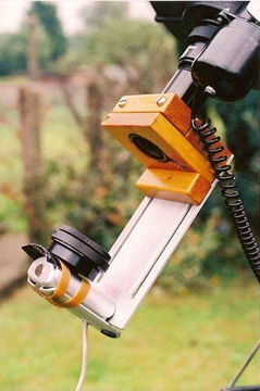
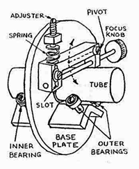
The restricted linear motion is achieved by mounting the eyepiece tube on rollers in a VEE formation using well known kinematic principles. This configuration eliminates side wobble and sticking, and the need to machine high precision bushings for the eyepiece tube in order to achieve accurate focusing action. Most CEM's use this system only, especially in conjunction with motorised focusing for CCD work. The linear motion is achieved by using a smooth pinion, which bears onto the focusing tube under light pressure.

[/et_pb_text][/et_pb_column][/et_pb_row][et_pb_row][et_pb_column type="1_3"][et_pb_text _builder_version="3.9"]

CEMImage1

[/et_pb_text][/et_pb_column][et_pb_column type="2_3"][et_pb_text _builder_version="3.9"]

Classical CEM

Features: VEE block ball race support rollers for eyepiece tube; hinged bracket; actuating lever. The smooth pinion bears directly on the eyepiece tube - one of a suite of removable and interchangeable eyepieces.

[/et_pb_text][/et_pb_column][/et_pb_row][et_pb_row][et_pb_column type="1_3"][et_pb_text _builder_version="3.9"]

CEMimage2

[/et_pb_text][/et_pb_column][et_pb_column type="2_3"][et_pb_text _builder_version="3.9"]

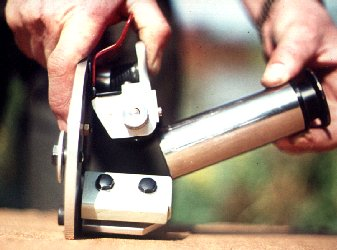
The quick release of the eyepiece tube: note the thumb tab action - this is an alternative to the sidelever.

[/et_pb_text][/et_pb_column][/et_pb_row][et_pb_row][et_pb_column type="1_3"][et_pb_text _builder_version="3.9"]

CEMImage3

[/et_pb_text][/et_pb_column][et_pb_column type="2_3"][et_pb_text _builder_version="3.9"]

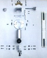
Exploded view of components to make a classical CEM. Scale rule is 300 mm.

[/et_pb_text][/et_pb_column][/et_pb_row][et_pb_row][et_pb_column type="4_4"][et_pb_text _builder_version="3.9"]

The quick action release is the second and more important function of the CEM. By lifting a lever the focusing pinion is moved away from the eyepiece tube, in order to release it. This enables rapid eyepiece changing in the dark. The focusing pinion is mounted on a hinged, spring loaded, bracket. The application of this mode is most useful for visual observations and camera work.

It's Home!

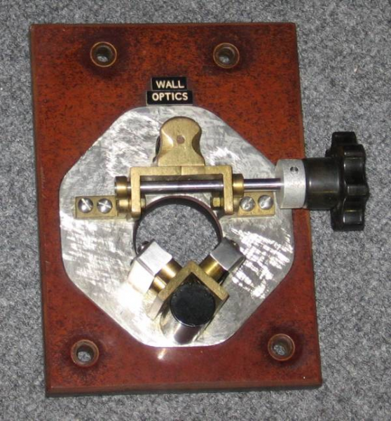
The original Crayford Eyepiece Mount has returned home! It has been donated by creator and telescope maker John Wall and is now on display in its special Perspex box at the Pavilion. Below is a picture of it.

CEMinage4

CEMJohnWall

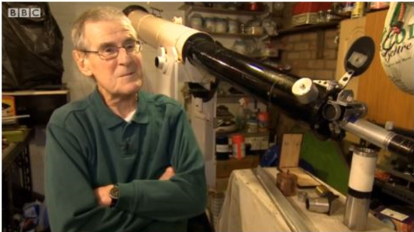
John Wall Interviewed by the BBC

[/et_pb_text][/et_pb_column][/et_pb_row][/et_pb_section]
HD209458

[et_pb_section bb_built="1"][et_pb_row][et_pb_column type="4_4"][et_pb_text _builder_version="3.9"]

HD 209458

HD 209458 is an 8th magnitude star in the constellation Pegasus. It is very similar to our Sun, and it is classified as a yellow dwarf (spectral class G0 V). The star is easily visible With good binoculars or small telescope.

Essential Details

Star Designation(s)

TYC 3198-1634-1 (TYC is also known as the Guide Star Catalog GSC)

Position

J2000 RA:22h 03m 10.7723s DEC:+18° 53' 03.548"

Magnitude (Vmag)

7.65

Expected variation

2%

Period

3.524748595 days

Results

The observations below were obtained on 2009 Aug 31 by carrying out time series photometry using a C9.25 SCT @ f10 with a MX916 camera, 'V' filter and 10 sec exposures. The 'V' filter in this instance was only used because the target star is so bright for CCD work. The conditions (typically) were less than ideal with intermittent cloud and a long stretch of cloud cover interfering with the observations. The top plot shows all of the data obtained. The next set is the same data but with all of the scatter removed. The bottom plot is this data average every five data points. The dip due to the transit can be seen in this plot.

hd209458bResultsMC01


[/et_pb_text][/et_pb_column][/et_pb_row][/et_pb_section]
Detecting an extrasolar planet – X0-2b

[et_pb_section fb_built="1" _builder_version="3.22" global_colors_info="{}"][et_pb_row _builder_version="3.25" background_size="initial" background_position="top_left" background_repeat="repeat" global_colors_info="{}"][et_pb_column type="4_4" _builder_version="3.25" custom_padding="|||" global_colors_info="{}" custom_padding__hover="|||"][et_pb_text _builder_version="4.14.7" hover_enabled="0" global_colors_info="{}" sticky_enabled="0"]

X0-2b

XO-2b is an example of a transiting hot Jupiter orbiting an early K dwarf star (TYC 3413-5-1) Vmag 11.2. Orbiting close in it has a period of approx. 2.615 days and takes approx. 2 hours to complete the transit. So far only partial light curves have been obtained due to weather conditions. However, with all of the observations plotted (Keith Rickard, Martin Crow) about their local transit times a phase curve has been generated.

Star Designation(s)

TYC 3413-5-1 (TYC is also known as the Guide Star Catalog GSC)

Position

J2000 RA: 7h48m06.47s DEC:+50°13'32.9"

Magnitude (Vmag)

11.2

Expected variation

0.02 Vmag

Period

2.615857±0.000005 days (~2hr transit)

XO-2b_phase_plot_transits

[/et_pb_text][/et_pb_column][/et_pb_row][/et_pb_section]
Julian Tworek’s Images of Mars

[et_pb_section bb_built="1"][et_pb_row][et_pb_column type="1_4"][et_pb_text _builder_version="3.9"]

Mars 2003-08-30

[/et_pb_text][et_pb_text _builder_version="3.9"]

Mars 2010-02-17

[/et_pb_text][/et_pb_column][et_pb_column type="1_4"][et_pb_text _builder_version="3.9"]

Mars 2003-07-10

[/et_pb_text][/et_pb_column][et_pb_column type="1_4"][et_pb_text _builder_version="3.9"]

Mars 2003-09-17

[/et_pb_text][/et_pb_column][et_pb_column type="1_4"][et_pb_text _builder_version="3.9"]

Mars 2003-09-17

[/et_pb_text][/et_pb_column][/et_pb_row][/et_pb_section]
Spectra Night

[et_pb_section fb_built="1" _builder_version="3.22" global_colors_info="{}"][et_pb_row _builder_version="3.25" background_size="initial" background_position="top_left" background_repeat="repeat" global_colors_info="{}"][et_pb_column type="4_4" _builder_version="3.25" custom_padding="|||" global_colors_info="{}" custom_padding__hover="|||"][et_pb_text _builder_version="4.14.7" global_colors_info="{}"]

Spectra Night - Thursday 13th August 2015

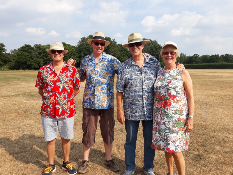
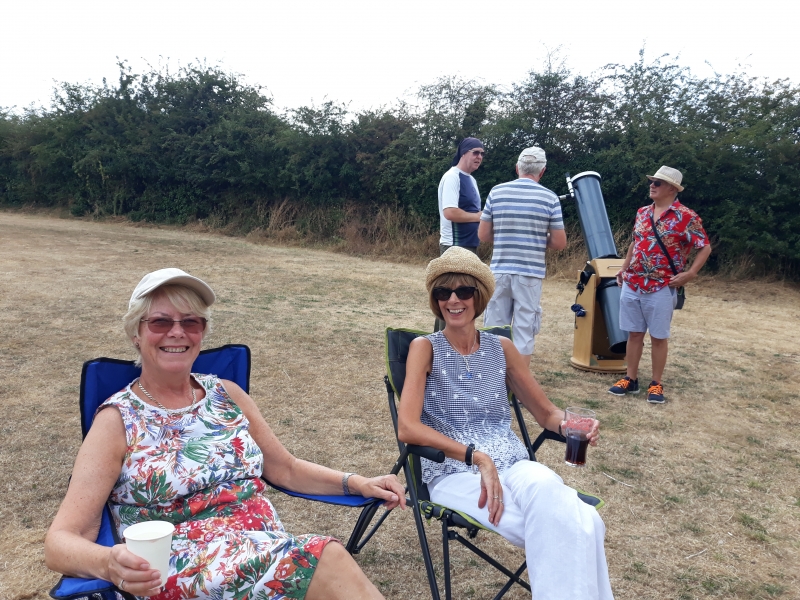
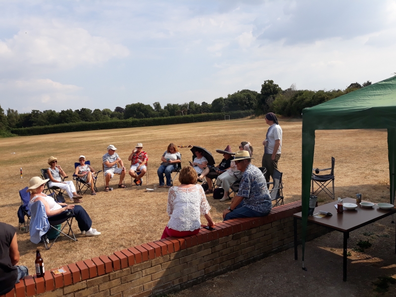
Below are a selection of fun photos from Honor Wheeler, Mike Rushton & Martin Crow of the evening member Debra Holton gave a talk about 'Spectra'.

Honor has also provided a great summary of evening too - Thank you Honor.

''As part of our Beginner primer talks given by members, our week 11 Informal meeting became a Spectra Spectacular! Member Debra Holton introduced us to the universe in light, the Electromagnetic Spectrum, the Doppler shift relating to redshift and blue shift and the distances & velocities of Stars and Galaxies.

The evening began with the members becoming acquainted with a number of interesting implements such as Diffraction gratings & glasses along with professional and homemade Spectroscopes.

Debra began with a simple introduction to the wavelengths of light from the Radio to Gamma rays and our very own rainbow of colours from our Sun, the visible spectrum. She then went on to describe how we see the elements that surround us, that atoms absorb and emit photons and in doing so how we can observe the emissions or absorption lines to learn what the distant Stars and Galaxies are made of.

After a little refresher on the spectra of stars and the Doppler shift using online resources, we progressed to a little more down to earth investigation.

Following on from a rather energetic display of the Doppler shift utilizing a hairdryer (you had to be there!) we moved on to the spectra of different light sources.

Thanks also go to member Gordon Collings, who many years ago rescued old laboratory spectroscopes, light boxes and lamps, as we had the opportunity to observe the spectra of a Mercury light & Sodium light and to bathe in the rather eerie light of a Sodium lamp.

Thank you to Debra for a fun and educational evening and to Gordon for his Light entertainment (Sorry couldn't resist!)''


[/et_pb_text][/et_pb_column][/et_pb_row][et_pb_row column_structure="1_4,1_4,1_4,1_4" _builder_version="3.25" background_size="initial" background_position="top_left" background_repeat="repeat" global_colors_info="{}"][et_pb_column type="1_4" _builder_version="3.25" custom_padding="|||" global_colors_info="{}" custom_padding__hover="|||"][et_pb_text admin_label="image" _builder_version="3.27.4" global_colors_info="{}"]

1stnight_02

[/et_pb_text][et_pb_text admin_label="image" _builder_version="3.27.4" global_colors_info="{}"]

SpectroscopyAug2015Attachment-1 (5)

[/et_pb_text][et_pb_text admin_label="image" _builder_version="3.27.4" global_colors_info="{}"]

SpectroscopyAug2015Attachment-1 (4) Large

[/et_pb_text][/et_pb_column][et_pb_column type="1_4" _builder_version="3.25" custom_padding="|||" global_colors_info="{}" custom_padding__hover="|||"][et_pb_text admin_label="image" _builder_version="3.27.4" global_colors_info="{}"]

SpectroscopyAug2015WP_001946

[/et_pb_text][et_pb_text admin_label="image" _builder_version="3.27.4" global_colors_info="{}"]

SpectroscopyAug2015Attachment-1 (2)

[/et_pb_text][et_pb_text admin_label="image" _builder_version="3.27.4" global_colors_info="{}"]

SpectroscopyAug2015Attachment-1 (3) Large

[/et_pb_text][/et_pb_column][et_pb_column type="1_4" _builder_version="3.25" custom_padding="|||" global_colors_info="{}" custom_padding__hover="|||"][et_pb_text admin_label="image" _builder_version="3.27.4" global_colors_info="{}"]

SpectroscopyAug2015MercuryAttachment-1

[/et_pb_text][et_pb_text admin_label="image" _builder_version="3.27.4" global_colors_info="{}"]

IMG_0697

[/et_pb_text][/et_pb_column][et_pb_column type="1_4" _builder_version="3.25" custom_padding="|||" global_colors_info="{}" custom_padding__hover="|||"][et_pb_text admin_label="image" _builder_version="3.27.4" global_colors_info="{}"]

SpectroscopyAug2015SodiumAttachment-1 (1)

[/et_pb_text][et_pb_text admin_label="image" _builder_version="3.27.4" global_colors_info="{}"]

WP_001945

[/et_pb_text][/et_pb_column][/et_pb_row][/et_pb_section]
TOP